ButchR

ButchR is an R package providing functions to perform non-negative matrix factorization and postprocessing using TensorFlow.

https://github.com/wurst-theke/ButchR

Citation

Andres Quintero, Daniel Hübschmann, Nils Kurzawa, Sebastian Steinhauser, Philipp Rentzsch, Stephen Krämer, Carolin Andresen, Jeongbin Park, Roland Eils, Matthias Schlesner, Carl Herrmann, ShinyButchR: interactive NMF-based decomposition workflow of genome-scale datasets, Biology Methods and Protocols, bpaa022.

ShinyButchR

We also provide an interactive R/Shiny app ShinyButchR to perform NMF and explore the results interactively. The live version can be used here: https://hdsu-bioquant.shinyapps.io/shinyButchR/

Or a pre-build image can be pulled from Docker: https://hub.docker.com/r/hdsu/shinybutchr

docker run --rm -p 3838:3838 hdsu/shinybutchr

Introduction

NMF (nonnegative matrix factorization) is a matrix decomposition method. A description of the algorithm and it’s implementation can be found e.g. in (Lee and Seung 1999). In 2003, Brunet et al. applied NMF to gene expression data (Brunet et al. 2003). In 2010, NMF, an R package implementing several NMF solvers was published (Gaujoux and Seoighe 2010). NMF basically solves the problem as illustrated in the following figure (Image taken from https://en.wikipedia.org/wiki/Non-negative_matrix_factorization):

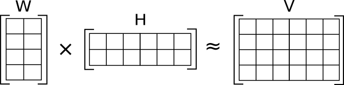
Here, V is an input matrix with dimensions n × m. It is decomposed into two matrices W of dimension n × l and H of dimension l × m, which when multiplied approximate the original matrix V. l is a free parameter in NMF, it is called the factorization rank. If we call the columns of W , then l corresponds to the number of signatures. The decomposition thus leads to a reduction in complexity if l < n, i.e. if the number of signatures is smaller than the number of features, as indicated in the above figure.

In 2015, Mejia-Roa et al. introduced an implementation of an NMF-solver in CUDA, which lead to significant reduction of computation times by making use of massive parallelisation on GPUs (Mejia-Roa et al. 2015). Other implementations of NMF-solvers on GPUs exist.

It is the pupose of the package ButchR described here to provide wrapper functions in R to these NMF-solvers in TensorFlow. Massive parallelisation not only leads to faster algorithms, but also makes the benefits of NMF accessible to much bigger matrices. Furthermore, functions for estimation of the optimal factorization rank and post-hoc feature selection are provided.

The ButchR package

The matrix decomposition results are stored in an S4 object called ButchR_NMF. ButchR provides functions to access the best factorzation after n initailization W and H matrices for a given factorzation rank.

NMF example - STAGE 1 preprocessing

For the tutorial we will use an RNA-seq dataset from labeled cell types of the human hematopoietic system, originally published on:

Corces MR, Buenrostro JD, Wu B, Greenside PG, Chan SM, Koenig JL, Snyder MP, Pritchard JK, Kundaje A, Greenleaf WJ, Majeti R, Chang HY. Lineage-specific and single-cell chromatin accessibility charts human hematopoiesis and leukemia evolution. Nat Genet 48, 1193–1203 (2016). https://doi.org/10.1038/ng.3646

In this session we will download and pre-process the data. The data will be downloaded as a counts matrix from GEO.

Preprocessing

Load required packages:

library(tidyverse)
library(viridis)
library(ComplexHeatmap)
library(DESeq2)
library(ButchR)
library(ggupset)
library(clusterProfiler)
library(msigdbr)
library(umap)
library(cowplot)

Download counts from GEO, select samples, and normalize data.

##----------------------------------------------------------------------------##
##                             Download counts                                ##
##----------------------------------------------------------------------------##
# set ftp url to RNA-seq data
ftp_url <- file.path("ftp://ftp.ncbi.nlm.nih.gov/geo/series/GSE74nnn/GSE74246",
                     "suppl/GSE74246_RNAseq_All_Counts.txt.gz")

read_delim_gz <- function(file_url) {
  con <- gzcon(url(file_url))
  txt <- readLines(con)
  return(read.delim(textConnection(txt), row.names = 1))
}

# read in data matrix
corces_rna_counts <- read_delim_gz(ftp_url)


##----------------------------------------------------------------------------##
##                        Data loading and sample QC                          ##
##----------------------------------------------------------------------------##

corces_rna_counts[1:5,1:5]

Click for Answer

##          X5852.HSC X6792.HSC X7256.HSC X7653.HSC X5852.MPP
## A1BG            14         9         1         5        13
## A1BG-AS1         3         0         1         0        27
## A1CF             0         0         0         0         0
## A2M             78       192        36        82        66
## A2M-AS1         71        76        52        86        49

dim(corces_rna_counts)

## [1] 25498    81

Remove leukemic and erythroblast samples:

corces_rna_counts <- corces_rna_counts[,-grep("Ery|rHSC|LSC|Blast", colnames(corces_rna_counts))]
dim(corces_rna_counts)

Click for Answer

## [1] 25498    46

Inspect correlation matrix:

cor_dm <- cor(corces_rna_counts)
Heatmap(cor_dm, col = magma(100), name = "Correlation")

Click for Answer

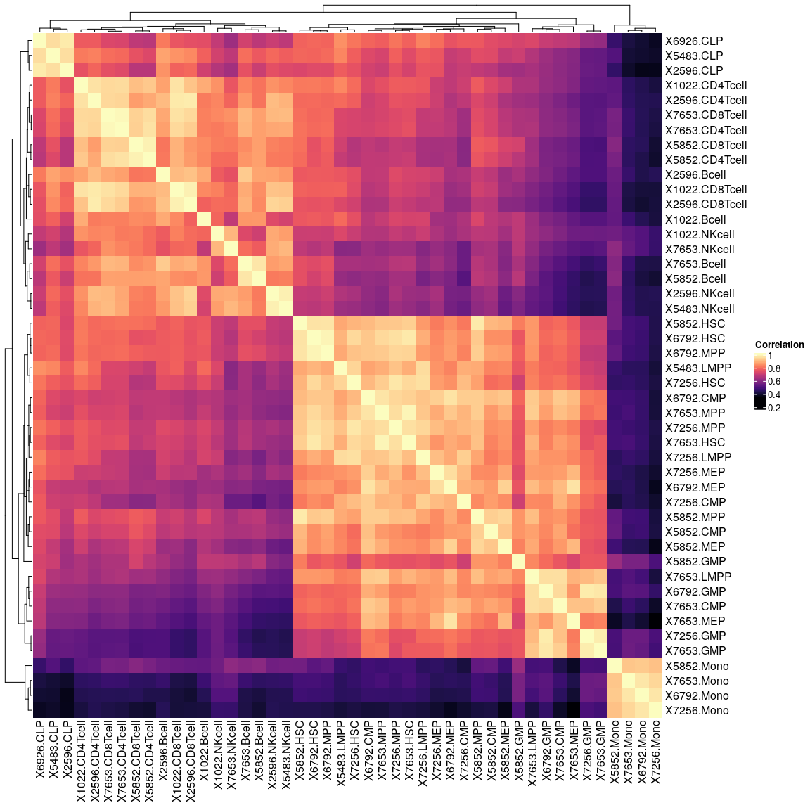
X5852.GMP is an outlier and will be removed, has much smaller library size as other GMPS:

rm(cor_dm)
corces_rna_counts <- corces_rna_counts[,-grep("X5852.GMP", colnames(corces_rna_counts))]

Remove rows with rowSum==0:

corces_rna_counts <- corces_rna_counts[!rowSums(corces_rna_counts) == 0,]

Normalize counts using DESeq2:

##----------------------------------------------------------------------------##
##                              Normalize counts                              ##
##----------------------------------------------------------------------------##

# do DESeq2 size factor normalization
sf <- estimateSizeFactorsForMatrix(corces_rna_counts)
corces_rna_counts <- t( t(corces_rna_counts) / sf )

# do +1 log2 transformation
corces_rna_norm <- apply(corces_rna_counts + 1, 2, log2)
rm(ftp_url, sf)

Format annotation data frame for future reference:

##----------------------------------------------------------------------------##
##                              Annotation                                    ##
##----------------------------------------------------------------------------##
# extract celltypes from colnames
col.anno <- gsub(".*\\.", "", colnames(corces_rna_norm))
col.anno[grep("NK", col.anno)] <- "NK"
col.anno[grep("CD4", col.anno)] <- "CD4"
col.anno[grep("CD8", col.anno)] <- "CD8"

# Define color vector
type.color <- setNames(c("#771155", "#AA4488", "#CC99BB", "#114477", "#4477AA", "#77AADD", 
                         "#117777", "#44AAAA", "#77CCCC", "#777711", "#AAAA44", "#DDDD77"),
                       c("HSC", "MPP", "LMPP", "CMP", "GMP", "MEP",
                         "CLP", "CD4", "CD8", "NK", "Bcell", "Mono"))

# Annotation data frame
corces_rna_annot <- data.frame(sampleID = colnames(corces_rna_norm),
                        Celltype = as.factor(col.anno),
                        color    = type.color[match(col.anno, names(type.color))],
                        row.names = colnames(corces_rna_norm),
                        stringsAsFactors = FALSE)

Dimension of transcriptome dataset (RNA-seq):

dim(corces_rna_norm)

Click for Answer

## [1] 21811    45

Preprocessing steps for the Corces 2016 ATAC-seq and to run iNMF can be found here