Test ButcherR-[BC]² Docker image

After running the ButcherR-[BC]² Docker image (see Run Docker image hdsu/butcher-bc2), you can run the following short example with a small leukemia dataset to test it.

Step 1 - Sign in to Rstudio

With the app open, sign in to RStudio using the following credentials:

• Username: hdsu
• Password: pass

Click for Answer

To start use "hdsu" as username and "pass" as password

Screen you should see after logging in to RStudio

Step 2 - Load packages

Run the following lines to load the required packages:

library(ButchR)
library(ComplexHeatmap)
library(viridis)
library(tidyverse)

Step 3 - Load leukemia data

Load the example data

data(leukemia)

Now we are ready to start an NMF analysis.

Step 4 - run NMF

The wrapper function for the NMF solvers in the ButchR package is run_NMF_tensor. It is called as follows:

k_min <- 2
k_max <- 4

leukemia_nmf_exp <- run_NMF_tensor(X = leukemia$matrix,
                                   ranks = k_min:k_max,
                                   method = "NMF",
                                   n_initializations = 10, 
                                   extract_features = TRUE)

Click for Answer

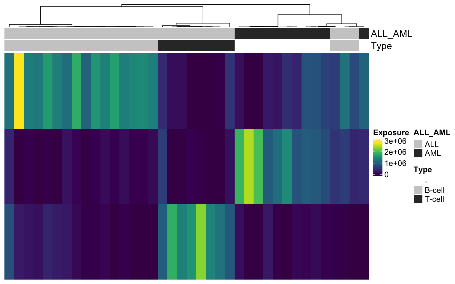
H matrix for k= 3

    ## [1] "2020-07-16 17:50:42 CEST"
    ## Factorization rank:  2 
    ## [1] "NMF converged after  75,123,64,69,58,126,141,83,54,87 iterations"
    ## [1] "2020-07-16 17:50:42 CEST"
    ## Factorization rank:  3 
    ## [1] "NMF converged after  154,79,90,87,66,84,76,151,115,102 iterations"
    ## [1] "2020-07-16 17:50:44 CEST"
    ## Factorization rank:  4 
    ## [1] "NMF converged after  108,189,202,108,121,76,104,150,110,132 iterations"
    ## No optimal K could be determined from the Optimal K stat

Depending on the choice of parameters (dimensions of the input matrix, number of iterations), this step may take some time. Note that the algorithm updates the user about the progress in the iterations.

Step 5 - Normalize W matrix

To make the features in the W matrix comparable, the factorization is normalized to make all columns of W sum 1.

leukemia_nmf_exp <- normalizeW(leukemia_nmf_exp)

Step 6 - Visualize the matrix H (exposures)

The matrices H may be visualized as heatmaps. We can define a meta information object and annotate meta data:

heat_anno <- HeatmapAnnotation(df = leukemia$annotation[, c("ALL_AML", "Type")],
                               col = list(ALL_AML = c("ALL" = "grey80", 
                                                      "AML" = "grey20"),
                                          Type = c("-" = "white",
                                                   "B-cell" = "grey80",
                                                   "T-cell" = "grey20")))

And now display the matrix H with meta data annotation:

#plot H matrix
tmp_hmatrix <- HMatrix(leukemia_nmf_exp, k = 3)
Heatmap(tmp_hmatrix,
        col = viridis(100),
        name = "Exposure",
        clustering_distance_columns = 'pearson',
        show_column_dend = TRUE,
        top_annotation = heat_anno,
        show_column_names = FALSE,
        show_row_names = FALSE,
        cluster_rows = FALSE)

Click for Answer

H matrix for k= 3