6. Differential Expression Analysis

The main advantage of using scRNA-Seq technologies is the possibility of assessing cell type specificity and heterogeneity, which is not possible while using bulk assays.

We should expect that some of the identified clusters in the UMAP might correspond to distinct cell types. The assignation of cell types identities is not always straightforward, some clusters might still contain some variability, and additionally, different clusters might correspond to the same cell type at a different functional, metabolic or cycling point.

Cell type profiling is generally done by assessing the expression of markers. This task can be done manually by inspecting markers in dimensional reduced data projected in UMAP or tSNE. It can also be done in a automatic manner scoring cells using gene signatures, which are lists of marker genes. Scores are generally based in the median expression of all the markers. Using scores has the advantage or reducing bias due to the arbitrary selection of markers.

Finding differential expressed markers is important for cluster profiling and identification. We will use the FindAllMarkers() function, which performs a statistical test comparing the distribution of gene expression values for each gene separately comparing one assigned cell type cluster (in this case the seurat_clusters column) vs the rest of cells.

First, we will set up the column used to define the clusters using the function Idents().

Idents(pbmc.filtered) <- pbmc.filtered$seurat_clusters

Now we can calculate the DEGs. There are several parameters for FindAllMarkers(), we will discuss logfc.threshold, min.pct and min.cells.feature that corresponds to the threshold of gene expression fold change, the minimum percentage of cells expressing the marker and the minimum of cells expressing (counts > 0) the feature. These parameters are used to filter out genes prior calculating DEGs. Lowering the values of these parameters will increase the sensibility of the method at the expense of increasing computation time.

pbmc.degs <- FindAllMarkers(pbmc.filtered, 
                            logfc.threshold = 1, 
                            min.pct = 0.05, 
                            min.cells.feature = 10, 
                            verbose = FALSE)

The output pbmc.degs consist of a data frame contanning the DEGs with p-vales, p-adjusted values and log fold change values for each gene as we can see next:

head(pbmc.degs)

##                 p_val avg_log2FC pct.1 pct.2    p_val_adj cluster     gene
## HLA-DRA  1.355148e-67  -4.415537 0.300 0.968 1.717379e-63       0  HLA-DRA
## HLA-DRB1 9.575850e-60  -3.310077 0.148 0.884 1.213547e-55       0 HLA-DRB1
## CD74     3.415369e-51  -3.122109 0.781 0.974 4.328297e-47       0     CD74
## HLA-DPB1 1.613117e-46  -3.269898 0.310 0.858 2.044303e-42       0 HLA-DPB1
## IL32     9.357132e-44   3.271671 0.808 0.110 1.185829e-39       0     IL32
## HLA-DRB5 2.825316e-43  -2.749389 0.084 0.684 3.580523e-39       0 HLA-DRB5

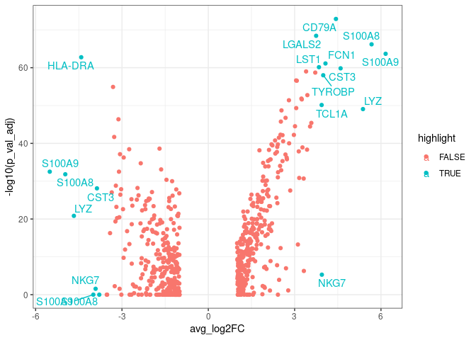
We can make a vulcano plot using ggplot:

library(ggplot2)
library(dplyr)         ## for handling data frames
library(ggrepel)

pbmc.degs %>%
  arrange(desc(abs(avg_log2FC))) %>%       ## Arranging genes by FC
  mutate(rank=1:nrow(pbmc.degs)) %>%        ## Ranking markers by FC
  mutate(highlight=ifelse(rank<20, TRUE, FALSE)) %>% ## highlighting top FC markers
  mutate(gene_label=ifelse(highlight==TRUE, gene, '')) %>% ## Adding labels for top markers
  ggplot(aes(x=avg_log2FC, y=-log10(p_val_adj),
             colour=highlight,
             label=gene_label)) +         ## adding labels for top markers
      geom_point() +
      geom_text_repel() +
      theme_bw()

Exercises

Compare the DEGs from the above shown results with that calculated using the 10X PBMC 250 cells downsample data clusters in the previous exercises

• Load the tsv file containing the calculated DEGs from above using the following url: https://raw.githubusercontent.com/caramirezal/caramirezal.github.io/master/bookdown-minimal/data/degs_10x_pbmc.tsv

• Calculate the DEGs using the downsampled 10X PBMC 250 cells data with the clusters obtained using your parameters

• Intersect both lists of genes

Previous Chapter | Next Chapter