5. Cell clustering

Detection of groups or cluster of cells is an important task in scRNA-Seq analysis. Seurat implements a clustering method based in KNN graphs and community detection using the Louvain algorithm. An important parameter for clustering is the resolution which can be set to increase/reduce the granularity of the clusters.

This method can be implemented by using the functions FindNeighbors() and FindClusters() as follows:

pbmc.filtered <- FindNeighbors(pbmc.filtered)
pbmc.filtered <- FindClusters(pbmc.filtered, 
                            resolution = 0.1, 
                            verbose = FALSE)

The results of the clustering are stored in the Seurat metadata slot, which can be accessed as a simple data.frame using the $ operator. A column vector containing each cluster for each cell is name seurat_cluster as shown next:

head(pbmc.filtered$seurat_clusters)

## AAAGAGACGGACTT-1 AAAGTTTGATCACG-1 AAATGTTGTGGCAT-1 AAATTCGAGCTGAT-1 
##                0                2                1                1 
## AAATTGACTCGCTC-1 AACAAACTCATTTC-1 
##                0                0 
## Levels: 0 1 2

There are 5 different clusters, labeled from 0 to 4 and stored like a factor. We can plot a frequency table of the number of cells assigned to each cluster by the algorithm.

table(pbmc.filtered$seurat_clusters) 

## 
##   0   1   2 
## 297  95  60

So, 297 cells were assigned to the cluster 0.

Exercises

Testing clustering: Try different different parameters for the clustering. For example, k.param in the FindNeighbors() function and higher levels of resolution.

Cluster visualization

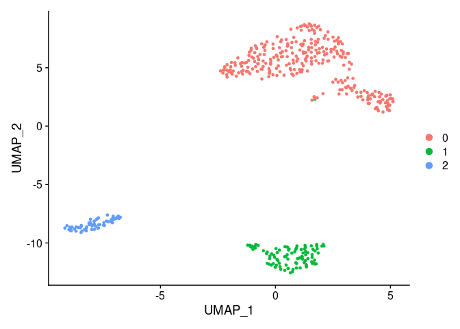
Transformations like PCA, tSNE or UMAP are used to project multidimensional data into 2D or 3D representations that can be visualized at the expense of the lose of information. tSNE and UMAP transformations aims to preserve global relations between sample points. We will use UMAPs to visualize the scRNA-Seq data from PBMC.

UMAP

We can use the RunUMAP function to calculate the UMAP transformation. The calculation of a UMAP projection can intensive computationally and is usually carried out on already dimensional reduced data using, for example, PCA. The RunUMAP from seurat by default will use the PCA reduced data, the parameter dims sets the number of dimensions, PCs that should be used, as we saw we can use 7 PCs which are the ones in which there is more variability.

pbmc.filtered <- RunUMAP(pbmc.filtered, 
                       dims = 1:7, 
                       verbose = FALSE)

After the calculation of the UMAP we can visualize it using the function DimPlot().

DimPlot(pbmc.filtered)

Exercise

• Perform UMAP visualization with the 10x PBMC 250 cells with your own set of parameters

• How does subsampling and parameters selection affects clustering?

Previous Chapter| Next Chapter