2. Quality control

Filtering cells with low sequencing quality is a very important step since it can greatly impact in further analysis. Quality check and control often requires to visualize and inspect samples in order to determine appropiate thresholds. Threshold values might vary from one dataset to another, so no hard threshold rule can be applied equally to every case.

We will examine the number of UMI counts, the number of RNA features and the percentage of reads of mitochondrial genes.

We will first calculate the percentage of UMI counts of reads mapped to mitochondrial genes. This step most be manually done since is based on a priori knowledge of which genes corresponds to mitochondrial genes. In this case, genes are annotated using human ensembl gene symbol annotations mitochondrial genes are annotated starting with a MT- string.

pbmc.seurat[["percent.mt"]] <- PercentageFeatureSet(pbmc.seurat, pattern = "^MT-")

Then, we can visualize the following metrics.

• Number of features - Correspond to the number of different mapped genomic features. For example, in the case of scRNA-Seq features corresponds to genes, in ATAC-Seq to genomic ranges, etc. High number of features can indicate doublets and empty cells. Usually between 1 and 30000.

• Number of counts - Number of mapped reads. It can also indicate the presence of doublets and empty droplet. It's generally correlated to the number of features. Usually between 1 and 20000.

• Percentage of mitochondrial genes - Percentage of mapped reads that are annotated to mitochondrial genes. The presence of high levels of % of mitochondrial genes can suggest that a cell have lost its membrane integrity or that the cytoplasm has been leaked off and only the mitochondria was retained. Usually a range from 0 to 10 is aceptable.

We can plot these metrics using the function VlnPlot() as follows:

VlnPlot(pbmc.seurat, features = c('nFeature_RNA', 'nCount_RNA', 'percent.mt'))

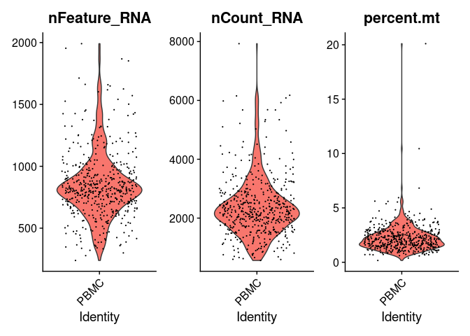
The violin plots show the values of the metrics for each cell along with an adjusted violin distribution.

Filtering out cells

Based on the previous violin plots we can define some thresholds and filter out cells using the subset function. In the following code we select cells having nFeatures < 1250, nCount < 4000 and percentage of reads mapped to mitochondrial genes < 5 percent.

pbmc.filtered <- subset(pbmc.seurat, 
                           nFeature_RNA < 1250 &
                                nCount_RNA < 4000 & 
                                    percent.mt < 5)

We can check the number of cell that passed the QC.

ncol(pbmc.filtered)

## [1] 452

Quizzes

How are the number of features and UMI counts related?
TIP: Use the function FeatureScatter, inspect the manual using ?function.

Answer:
```r FeatureScatter(pbmc, feature1 = "nCount_RNA", feature2 = "nFeature_RNA") ```

We observe as expected a linear relation between the number of UMI counts and the features recorded.

Exercises

Performing your own QC

Perform a QC using the downsampled 10x PBMC 250 cells data

• Calculate and visualize QC metrics
• Filter out cells based on the calculated values

Normalization

There are several methods for normalization of scRNA-Seq data. A commonly used strategy is the log normalization which basically corrects sequencing deep in cells by dividing each feature by the total number of counts and then multiplied the result by a factor, usually 10000, and finally the values are log transformed.

Log normalization can be implemented by using the NormalizeData() function.

pbmc.filtered <- NormalizeData(pbmc.filtered)

Then, in order to make genes measurements more comparable log transformed values are scaled in a way that the media is equal to zero and the variance is equal to 1 as follows:

pbmc.filtered <- ScaleData(pbmc.filtered)

Previous Chapter | Next Chapter